|
⇤ ← Revision 1 as of 2021-02-17 12:10:01
Size: 6640
Comment:
|
Size: 6634
Comment:
|
| Deletions are marked like this. | Additions are marked like this. |
| Line 16: | Line 16: |
| ===== NWChem with DPLOT ===== | == NWChem with DPLOT == |
Visualising the Molecular Orbitals
Here we will use the NWChem program together with the Avogadro program to visualise the molecular orbitals.
Important You will need to have Avogadro installed on your laptop for this to work. And you will need to be able to download files from comanche to your laptop.
- Avogadro is free and is cross-platform so install it on your laptop.
To download files from comanche you may use sftp from your laptop. Or use mobaxterm to do the file transfer for you. As comanche and poset share the home file system, you can just as well transfer the file from poset to your laptop.
NWChem with DPLOT
Important See the full description of the ''DPLOT'' module on the NWChem site.
We will use the DPLOT module in NWChem to create Gaussian Cube files. These are really wasteful and simple-minded files that store graphical information on a grid of points. You set the quality of the grid, and then the code calculates the relevant quantity and stores it in the file. These files tend to be large. Worse, you will need a separate file for each orbitals!
Here is an example for H$_2$O:
Memory 500 mb

charge 0
Geometry units bohr
  O     0.0000000000    0.0000000000    0.0000000000
  H1   -1.4536519600    0.0000000000   -1.1216873200
  H2    1.4536519600    0.0000000000   -1.1216873200
End

Basis "ao basis" spherical
  H  library  STO-3G
  O  library  STO-3G
End

Title "H2O STO-3G "

scf
  Singlet
  vectors output h2o.movecs
end

dplot
  Title H2O
  vectors h2o.movecs
  LimitXYZ  units Angstrom
    -4.0  4.0   40
    -4.0  4.0   40
    -4.0  4.0   40
  spin total
  gaussian
  Orbitals
  5
  1 2 3 4 5
  output density.cube
end

task scf energy
task dplot
The DPLOT commands are as follows
Title H2O : this should be self-explanatory.
vectors h2o.movecs: Here we have saved the molecular orbital coefficients in file h2o.movecs, so these are now read in.
LimitXYZ: This command is followed by three lines that specify the extent of the Cube grid as follows:
LimitXYZ
   Xmin   Xmax   Points_for_X
   Ymin   Ymax   Points_for_Y
   Zmin   Zmax   Points_for_Z
Note that the grid does not have to be in the shape of a cube. It may be a rectangle. The important part is to make it large enough to enclose the molecular orbital and yet not too large that the spacing between points becomes too large. Units for the grid can be set using the units command.
Spin total: Tells NWChem whether to include spin up or down or the sum.
GAUSSIAN: Says to create a Cube file in the Gaussian format.
Orbitals: Allows you to specify what to display:
ORBITALS  [VIEW]
  <integer number of orbitals>
  <integer list of orbitals>


For the density arising from orbitals 1 to 5 use:

Orbitals
  5
  1 2 3 4 5

For the density arising from orbitals 4 and 5 only use:

orbitals
  2
  4 5

For molecular orbital 3 use:

Orbitals view
  1
  3

Note that molecular orbitals must be specified one at a time. So to visualise the first MO use:

Orbitals view
  1
  1
OUTPUT : Specifies the name of the output file.
TASK DPLOT : Tells NWChem to run the DPLOT code.
You can combine many DPLOT commands in a single file as follows: h2o-sto3g-dplot.nw
Memory 500 mb

charge 0
Geometry units bohr
  O     0.0000000000    0.0000000000    0.0000000000
  H1   -1.4536519600    0.0000000000   -1.1216873200
  H2    1.4536519600    0.0000000000   -1.1216873200
End

Basis "ao basis" spherical
  H  library  STO-3G
  O  library  STO-3G
End

Title "H2O STO-3G "

scf
  Singlet
  vectors output h2o.movecs
end

dplot
  Title H2O
  vectors h2o.movecs
  LimitXYZ
    -4.0  4.0   40
    -4.0  4.0   40
    -4.0  4.0   40
  spin total
  gaussian
  Orbitals
  5
  1 2 3 4 5
  output density.cube
end

task scf energy
task dplot

dplot
  Title H2O
  vectors h2o.movecs
  LimitXYZ
    -4.0  4.0   40
    -4.0  4.0   40
    -4.0  4.0   40
  spin total
  gaussian
  Orbitals
  1
  5
  output density-orb5.cube
end
task dplot

dplot
  Title H2O
  vectors h2o.movecs
  LimitXYZ
    -4.0  4.0   40
    -4.0  4.0   40
    -4.0  4.0   40
  spin total
  gaussian
  Orbitals view
  1
  5
  output mo-5.cube
end
task dplot

dplot
  Title H2O
  vectors h2o.movecs
  LimitXYZ
    -4.0  4.0   40
    -4.0  4.0   40
    -4.0  4.0   40
  spin total
  gaussian
  Orbitals view
  1
  4
  output mo-4.cube
end
task dplot

dplot
  Title H2O
  vectors h2o.movecs
  LimitXYZ
    -4.0  4.0   40
    -4.0  4.0   40
    -4.0  4.0   40
  spin total
  gaussian
  Orbitals view
  1
  3
  output mo-3.cube
end
task dplot
Here we first calculate the density arising for all occupied MOs (1, 2, 3, 4 & 5), then the density from MO 5 only. This is followed by the actual MOs (3, 4 & 5).
Run this as usual using: Run the job
 $ mpirun.mpich -np 1 nwchem h2o-sto3g-dplot.nw >& h2o-sto3g-dplot.out

  If it has run correctly you will have 5 Cube files in this directory.
Avogadro
Now that we have the MOs, how do we display them?
- Start Avogadro
File -> Open
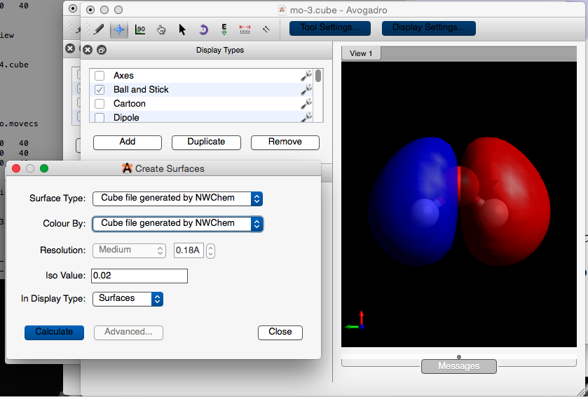
Select Cube file: mo-3.cube.
- You should now see a stick figure of a water molecule.
Extensions -> Create Surfaces...
- This gives you a new menu in a window.
Select: Surface Type : Cube file generated by NWChem
Select: Color By : Cube file generated by NWChem
Click on: Calculate
- Do you get the following?

This MO is the third one and is occupied by two electrons. NWChem defines it as: MO 3
 Vector    3  Occ=2.000000D+00  E=-6.106389D-01  Symmetry=a'
              MO Center= -1.5D-01, -5.6D-16, -4.9D-32, r^2= 8.4D-01
   Bfn.  Coefficient  Atom+Function         Bfn.  Coefficient  Atom+Function
  ----- ------------  ---------------      ----- ------------  ---------------
     4      0.605698  1 O  py                 6     -0.445851  2 H  s
     7      0.445851  3 H  s
Can you see why this looks like the picture above?
