|
⇤ ← Revision 1 as of 2021-02-17 13:14:13
Size: 19308
Comment:
|
Size: 19284
Comment:
|
| Deletions are marked like this. | Additions are marked like this. |
| Line 6: | Line 6: |
| This material is based on the paper: {{:ajm:teaching:electronic-structure:ammonia_monohydrate_high_pressure_phases_griffithsmfpn12_jcp137.pdf|G. Griffiths, A. J. Misquitta, R. J. Needs, C. J. Pickard and A. D. Fortes ``Theoretical study of ammonia monohydrate at pressures up to 12 GPa'' J. Chem. Phys. 137, 064506 (2012)}}. | This material is based on the paper: [[attachment:ammonia_monohydrate_high_pressure_phases_griffithsmfpn12_jcp137.pdf|G. Griffiths, A. J. Misquitta, R. J. Needs, C. J. Pickard and A. D. Fortes ``Theoretical study of ammonia monohydrate at pressures up to 12 GPa'' J. Chem. Phys. 137, 064506 (2012)]]. |
Contents
Ammonia Monohydrate
This material is based on the paper: G. Griffiths, A. J. Misquitta, R. J. Needs, C. J. Pickard and A. D. Fortes ``Theoretical study of ammonia monohydrate at pressures up to 12 GPa'' J. Chem. Phys. 137, 064506 (2012).
Crystal Structure
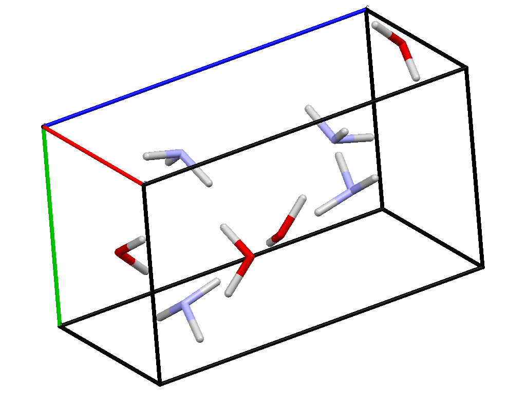
There are two phases: the molecular:
And the ionic:
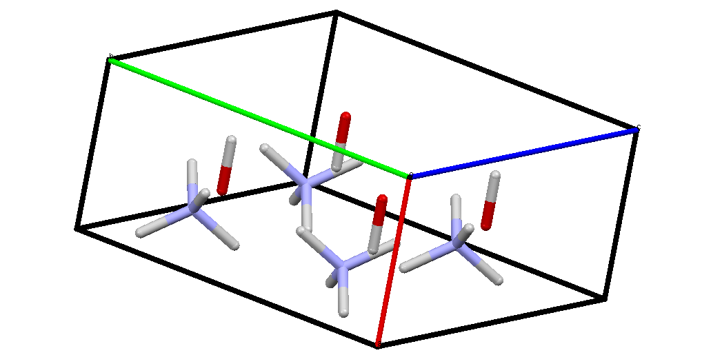
These are possibly more easily viewed using the ShelX files. I cannot upload them here so they are on this page.
The ionic phase becomes more stable than the molecular phase at a pressure of more than 10 GPa (GPa = Giga Pascal).
Features of AMH
Important This is just a summary of some of the results described at length in the introduction of the paper. Please look there for more details.
Ammonia monohydrate (AMH = NH$_{3}\cdots$H$_2$O) exists as at least six different polymorphs over a pressure range of 0 to 9 GPa and temperature range of 170 to 295K.
- Planetary significance: large amounts of water and ice accreted into the satellites of gas giants.
- Contains weak hydrogen bonds as well as dispersion interactions. This poses a challenge to density functional methods (more on this in the class).
- The structures of AMH-III and AMH-IV remain to be determined.
Griffiths //et al.// show that molecular AMH phases are unstable with respect to the formation of ionic ammonium hydroxide (NH$_4^+\cdots$OH$^-$) proton transfer phases at pressures of about 2.8 GPa.
- However, no experimental evidence for such phases has been found at the time of the paper.
- Including dispersion forces (not included in DFT - this will have to wait for the second lecture on DFT) to the PBE density functional (PBE is a commonly used density functional) has a significant effect on the volumes and relative enthalpies of the phases in this system.
- But PBE poorly describes the proton transfer ionic phase.
- AMH structures have been found using the ab initio random structure search (AIRSS) method.
PBE Enthalpies
Here are PBE and PBE+D(G06) relative enthalpies for a few phases of AMH. $\Delta H$ values are presented w.r.t. the experimental AMH-II phase. So values less than this phase, i.e., a more stable phase, would appear negative on these plots. 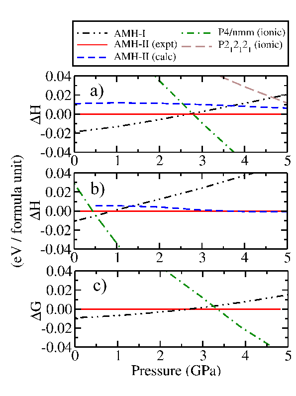 Enthalpies per formula unit (f.u.) of AMH structures relative to AMH-II calculated with: a) the PBE functional, b) the PBE functional and G06 semi-empirical dispersion correction. The Gibbs free energy per f.u. of AMH structures relative to that of AMH-II is shown in c), calculated with the PBE functional including vibrational motion at 175 K. AMH-II (expt) denotes the structure found in experiment while AMH-II (calc) denotes the structure found in the AIRSS study reported in Fortes et al. 2009.
Notice the following:
The stability range of AMH-II between the AMH-I and ionic $P4/nmm$ phases predicted by the PBE functional is very small ($\sim$0.01 GPa).
- However, experiments have shown that the transition from AMH-I to AMH-II takes place at around 0.5 GPa, and then from AMH-II to AMH-IV (whose structure is presently unknown) at around 2.2 GPa at 170 K.
PBE calculations predict the ionic $P4/nmm$ phase to be thermodynamically stable across a broad region of the high pressure phase diagram.
The relative enthalpy of the ionic $P4/nmm$ structure, computed with the PBE functional, is shown in Fig. 1(a). We find that its enthalpy declines very rapidly with pressure, such that it allows AMH-II only the narrowest window of thermodynamic stability (∼0.01 GPa) with the PBE functional, and no region of stability at all with PBE+G06.
- This result is difficult to reconcile with the existing experimental results, which clearly demonstrate a wide region (at least 2 GPa) over which AMH-II is stable.
Important
We need to understand (theoretically and numerically):
Why PBE results in an apparently over-stabilised $P4/nmm$ phase.
Why the dispersion correction is essential for both phases (see below) but nevertheless even more over-stabilises the $P4/nmm$ phase.
Properties of the $P4/nmm$ phase
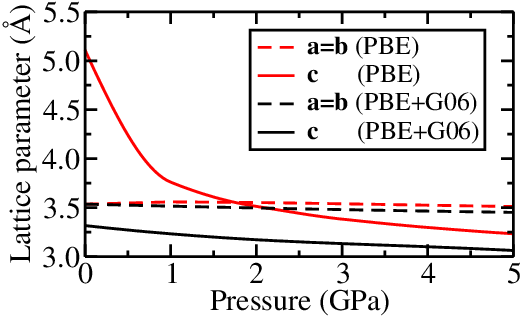 The effect of the dispersion correction to PBE is minimal on the $a$ and $b$ lattice parameters. But the effect on the $c$ parameter is huge. The dispersion correction dramatically reduces this parameter. How can we understand this?
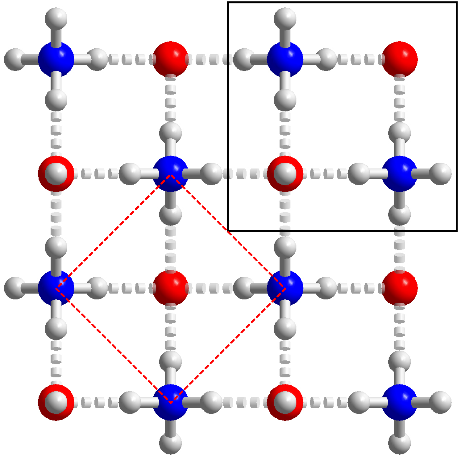 The ionic $P4/nmm$ phase viewed along the $c$-axis. This structure comprises sheets of ions hydrogen-bonded together (dashed rods) donated by the ammonium ions to the hydroxide. The hydrogen atom of the hydroxide ion points directly along the c-axis and does not appear to participate in a hydrogen bond. Hence, the layers are not H-bonded to one another and consequently the structure exhibits a large compressibility along the c-axis.
Important
How can we understand why the $P4/nmm$ phase is so compressible along the $c$ axis? How will we show this numerically?
Approach
We will not be performing any solid-state calculations in this course. While the theoretical methods required are the same as those we have studied here, the numerical and algorithmic details are quite different. Instead we will attempt to analyse the problem by breaking it down into smaller parts and analysing the parts in detail.
We will do this by extracting dimers from the molecular AMH-I and ionic $P4/nmm$ phases. This takes a while to get right: how do we choose dimers? The choice is not unique and we may, in some cases, need to extract many kinds before we get a complete picture. What helps is the high symmetry in the crystal. Here, using my own understanding of intermolecular interactions (a subject we will cover in the next lecture), I was able to figure out what were the best dimer choices: basically it boiled down to recognising the strongest bonds in the system. These are typically hydrogen-bonds.
Here is the dimer from the molecular AMH-I phase: 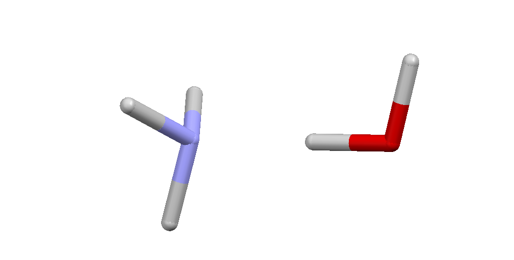 These are the coordinates of the molecules in this orientation, but with the Nitrogen and Oxygen atoms both at the origin:
AMH-I H-bonded dimer : Reference
Molecule NH3
  Units ANGSTROM
    1  N1          7.00     0.00000000    0.00000000    0.00000000
    2  H1          1.00     0.98600692    0.00000000   -0.30465448
    3  H2          1.00    -0.46058281    0.84107528   -0.38141820
    4  H3          1.00    -0.46058281   -0.84107528   -0.38141820
End

Molecule H2O
  Units ANGSTROM
    1  O1          8.00     0.00000000    0.00000000    0.00000000
    2  H1          1.00     0.00000000    0.00000000   -1.03900000
    3  H2          1.00    -0.96568028    0.00000000    0.27836416
End
To form the dimer shown above we need to translate H2O by 3.0 Angstrom along the $z$-axis, i.e., we need to add $(0.0,0.0,3.0)$ to all atomic coordinates in H2O.
This makes it easy to do what we need to do next: we need to calculate interaction energies (as we did for the argon dimer) at a variety of separations. To generate these separations all we need to is alter the $z$-coordinates of the atoms in H2O.
And here is the dimer from the ionic $P4/nmm$ phase: 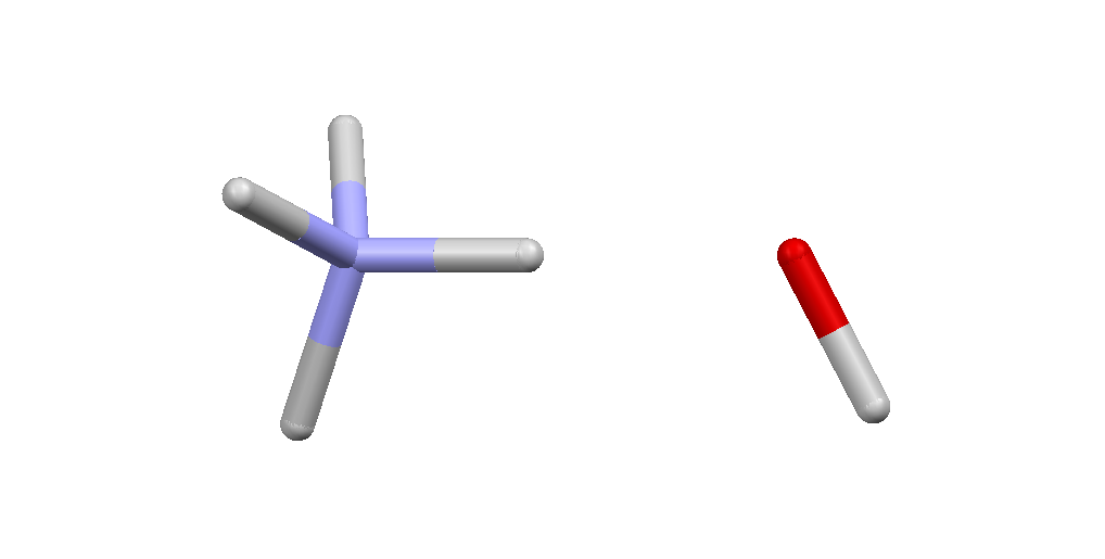 And here are the coordinates of the two molecules in their reference geometry:
Molecule NH4
  Units ANGSTROM
    1  N1          7.00     0.00000000    0.00000000    0.00000000
    2  H2          1.00     0.00000000    0.00000000    1.06400000
    3  H3          1.00     0.00000000    0.98079042   -0.41248777
    4  H4          1.00     0.85956263   -0.53732297   -0.32331426
    5  H5          1.00    -0.85956263   -0.53732297   -0.32331426
End

Molecule OH
  Units ANGSTROM
    1  O1          8.00     0.00000000    0.00000000    0.00000000
    2  H1          1.00     0.00000000    0.88002486    0.41036233
End
To form the dimer shown above we need to translate the OH ion along the $z$-axis by 2.3 Angstroms, i.e., add $(0.0,0.0,2.3)$ to the O1 and H1 coordinates.
Task 1 : Determine the reference energies
- We will use MP2 as our reference. Griffiths et al. used CCSD(T), but this is not necessary as CCSD(T) is pretty close to MP2 for these systems.
Our goal is to calculate a potential energy scan (1D cut through the 6D PES of these dimers) for each of these dimers. So we need to set up NWChem scans for each of these dimers. The procedure will be similar to what we did for Ar$_2$.
- Before performing the scans, create sample input files for each of these dimers. Get them checked. Or check them yourself using a small basis set for the tests (cc-pvdz will do).
Keep in mind that for the $P4/nmm$ dimer, the molecules are ionic, so we need to tell NWChem that they are charged. How will you do this?
- Run the calculations and calculate the interaction energies at these geometries. I have reference values you can compare your results to.
Setting up your NWChem input files
- You need to get the geometry right. The geometries given above need to be modified: one of the molecules will have to be translated otherwise you will have one over the other!
Basis sets: The smallest basis you can sensibly use is the cc-pvdz.
scratch_dir: Don't forget to define it!!!
Charged systems: Define the charge in after each set geometry command.
set geometry "NH4+OH"
charge 0
task mp2
unset geometry "NH4+OH"

scf; vectors atomic; end

set geometry "OH+ghost"
charge -1
task mp2
unset geometry "OH+ghost"

scf; vectors atomic; end

set geometry "NH4+ghost"
charge +1
task mp2
unset geometry "NH4+ghost"
- SCF convergence: You need the following line before each monomer calculation. Else the SCF may not converge at all, or will converge to an excited state. Try a calculation without it and see what happens.
scf; vectors atomic; end
Task 2 : Reference PESs for the dimers
What we really want is the interaction energy profile. That is, $E_{\rm int}(R)$ for a set of $R$ values. Here $R$ will be the O..N separations. That is, it will be the amount you've translated the H2O or OH molecules along the $z$ axis.
For the AMH-I dimer, perform MP2 calculations for $R=2.4, 2.6, 2.8, 3.0, 3.2, 3.4, 4.0, 5.0, 6.0, 10.0$ Angstrom.
For the $P4/nmm$ dimer do the same for $R=1.7, 2.1, 2.3, 2.5, 2.7, 3.1, 4.0, 5.0, 10.0, 20.0$ Angstrom.
- Calculate the interaction energies and plot them.
- These will be your reference energies against which we will compare DFT energies.
Here's a Python script that will perform a batch calculation for the AMH-I dimer:
# This may need to be /usr/bin/python2.7 on comanche

import argparse, numpy, subprocess, re, sys, os
import numpy, re, sys, subprocess
#import matplotlib.pyplot as plt

# Parse command-line arguments

parser = argparse.ArgumentParser(description = """
Create a set of NWChem input files for the Ar2 dimer, run NWChem on them, and
parse the output for interaction energy.
""")
parser.add_argument("-m", "--min", dest="minR", type=float, default=1.,
                    help="minimum Ar separation in A")
parser.add_argument("-M", "--max", dest="maxR", type=float, default=5.,
                    help="maximum Ar separation in A")
parser.add_argument("-d", "--delta", dest="deltaR", type=float, default=0.5,
                    help="step size for Ar separation in A")
parser.add_argument("-o", "--output", dest="output", type=str, default="output.txt",
                    help="output text file")
parser.add_argument("-np", "--nproc", dest="nproc", type=int, default=1,
                    help="Number of processors to be used.")
parser.add_argument("-b", "--basis", dest="basis", type=str, default="aug-cc-pvtz",
                    help="basis set used in calculation")

args = parser.parse_args()

nwchem_dir = os.environ["NWCHEM_TOP"]
username = os.environ["USER"]
nproc = args.nproc


# I have commented out the uniform grid:
#positions = numpy.arange(args.minR, args.maxR + 0.00001, args.deltaR)
# Instead, use a non-uniform grid specific to your system:
positions = numpy.array([1.7,2.1,2.3,2.5,2.7,3.1,4.0,5.0,10.0,20.0])

print "Basis set ",args.basis
print "positions = ", positions
print "Output to : ",args.output
print "Number of processors : ",nproc
output = open(args.output,'w')


# Conversion factor:
au2cm = 219474.631371
au2kJ = 2625.499

# Construct input files

input_file_template = """
title "NH3..H2O BSSE corrected MP2 interaction energy"

scratch_dir /scratch/HDD_2T/{user}/nwchem

geometry units angstrom "NH3+H2O"
  N       0.00000     0.00000     0.00000
  H1      0.98601     0.00000    -0.30465
  H2     -0.46058     0.84108    -0.38142
  H3     -0.46058    -0.84108    -0.38142
  O       0.00000     0.00000     {RzO}
  H4      0.00000     0.00000     {RzH4}
  H5     -0.96568    -0.00000     {RzH5}
end

geometry units angstrom "NH3+ghost"
  N       0.00000     0.00000     0.00000
  H1      0.98601     0.00000    -0.30465
  H2     -0.46058     0.84108    -0.38142
  H3     -0.46058    -0.84108    -0.38142
  BqO     0.00000     0.00000     {RzO}
  BqH     0.00000     0.00000     {RzH4}
  BqH    -0.96568    -0.00000     {RzH5}
end

geometry units angstrom "ghost+H2O"
  BqN       0.00000     0.00000     0.00000
  BqH       0.98601     0.00000    -0.30465
  BqH      -0.46058     0.84108    -0.38142
  BqH      -0.46058    -0.84108    -0.38142
  O         0.00000     0.00000     {RzO}
  H4        0.00000     0.00000     {RzH4}
  H5       -0.96568    -0.00000     {RzH5}
end

basis
 N   library    {basis}
 H1  library    {basis}
 H2  library    {basis}
 H3  library    {basis}
 O   library    {basis}
 H4  library    {basis}
 H5  library    {basis}
 BqN   library  N  {basis}
 BqH   library  H  {basis}
 BqO   library  O  {basis}
end

set geometry "NH3+H2O"
charge 0
task mp2
unset geometry "NH3+H2O"

scf; vectors atomic; end

set geometry "NH3+ghost"
charge 0
task mp2
unset geometry "NH3+ghost"

scf; vectors atomic; end

set geometry "ghost+H2O"
charge 0
task mp2
unset geometry "ghost+H2O"

"""

# z coordinates for O, H4 and H5 : H2O will be translated along the z-axis
# Units: Angstrom
zO  =  0.0
zH4 = -1.03900
zH5 =  0.27836

# Regular expressions to find the right lines in the file

scf_re = re.compile("SCF energy\s+(-?[0-9]+.[0-9]+)")
mp2_re = re.compile("Total MP2 energy\s+(-?[0-9]+.[0-9]+)")

# Dictionary to store the energies we find

energies = {}

# Main loop through different position values

for delta_z in positions:
    print "Current position = ",delta_z
    input_file_name = "in-R{0:5.3f}.nw".format(delta_z)
    output_file_name = "out-R{0:5.3f}.out".format(delta_z)

    # Write input file
    Rz_O  = zO + delta_z
    Rz_H4 = zH4 + delta_z
    Rz_H5 = zH5 + delta_z
    RzO  = """{0:10.6f}""".format(Rz_O)
    RzH4 = """{0:10.6f}""".format(Rz_H4)
    RzH5 = """{0:10.6f}""".format(Rz_H5)
    input_file = open(input_file_name, "w")
    input_file.write(input_file_template.format(RzO=RzO,RzH4=RzH4,RzH5=RzH5,user=username,basis=args.basis))
    input_file.close()

    # Run NWChem

    output_file = open(output_file_name, "w")
    subprocess.call(["mpirun.mpich","-np",str(nproc),"nwchem", input_file_name],
                                                stdout=output_file, stderr=subprocess.STDOUT)
    output_file.close()

    # Read output file back in

    output_file = open(output_file_name, "r")
    scf_energies = []
    mp2_energies = []
    for line in output_file:
        scf_match = scf_re.search(line)
        if scf_match:
            scf_energies.append(float(scf_match.group(1)))
        else:
            mp2_match = mp2_re.search(line)
            if mp2_match:
                mp2_energies.append(float(mp2_match.group(1)))
    output_file.close()

    if not (len(scf_energies) == 3 and len(mp2_energies) == 3):
        print "Apparent error in output file! {:d} SCF energies and {:d} MP2 energies found.".format(
            len(scf_energies), len(mp2_energies))
        sys.exit(1)

    energies[delta_z] = scf_energies + mp2_energies
    scf_dimer    = energies[delta_z][0]
    scf_monomerA = energies[delta_z][1]
    scf_monomerB = energies[delta_z][2]
    mp2_dimer    = energies[delta_z][3]
    mp2_monomerA = energies[delta_z][4]
    mp2_monomerB = energies[delta_z][5]
    scf_interaction = scf_dimer - scf_monomerA - scf_monomerB
    mp2_interaction = mp2_dimer - mp2_monomerA - mp2_monomerB
    print "Eint[SCF] = ",scf_interaction*au2kJ
    print "Eint[MP2] = ",mp2_interaction*au2kJ

# prepare plots

scf_dimer = numpy.array([energies[p][0] for p in positions])
scf_monomerA = numpy.array([energies[p][1] for p in positions])
scf_monomerB = numpy.array([energies[p][2] for p in positions])
mp2_dimer = numpy.array([energies[p][3] for p in positions])
mp2_monomerA = numpy.array([energies[p][4] for p in positions])
mp2_monomerB = numpy.array([energies[p][5] for p in positions])

scf_interaction = scf_dimer - scf_monomerA - scf_monomerB
mp2_interaction = mp2_dimer - mp2_monomerA - mp2_monomerB

# convert to kJ/mol
scf_interaction = au2kJ*scf_interaction
mp2_interaction = au2kJ*mp2_interaction

output.write(('%10s '*9 + '\n') %
             ("   R    ","SCF monoA","SCF monoB","SCF dimr","SCF int ",
                         "MP2 monoA","MP2 monoB","MP2 dimr","MP2 int "))

for i in range(len(positions)):
    output.write(('%10.6f '*9 + '\n') %
    (positions[i],
    scf_monomerA[i], scf_monomerB[i], scf_dimer[i], scf_interaction[i],
    mp2_monomerA[i], mp2_monomerB[i], mp2_dimer[i], mp2_interaction[i]))

output.close()
Save this script as AMH-I-batch_MP2_nwchem.py. Make the script executable using
$ chmod +x AMH-I-batch_MP2_nwchem.py
The arguments to the script are found using the --help flag.
$ ./AMH-I-batch_MP2_nwchem.py --help
- Note that although the script appears to allow you to set the range of points at which the scan is to be done, these lines are commented out in the code and the points are hard-coded.
Run this using the aug-cc-pvdz basis set. Make sure that the reference energies you obtain agree with those in Griffiths et al.
Important
You will need to write a similar script for the $P4nmm$ dimer.
