Water potential Notes: Rory

See also:

1. Potential Development using CamCASP

2. Charge-Transfer

3. Polarization & Polarization Models

4. Rory's continued notes on Water

Friday 12th

I can't actually work out how to copy a graph onto my computer from comanche. I have produced graphs for the three anchors strengths set to 0.001 with the Boltzmann parameter set to 10, 20, 30 and 40. "10" isn't very good, I think you said it would be too low, I'd say "40" is slightly better than "20" although there isn't much difference between them. I still have to finish off producing new outputs to replace the ones made incorrectly (without remembering to remove the weights column) however the orient files are ready with the correct Boltzmann parameter. Once this is done I should vary the anisotropic anchor value some more.

Monday 15th

With $\alpha$ and $iso$ anchor strengths set to $0.01$ each the "best" plot seems to be quite well reproduced, and this is actually still quite close to letting the $\alpha$ parameter take $0.1$ whilst leaving the $iso$ parameter at $0.01$. For the aisotropic anchor, there is no reason to go below $0.01$ but that's probably the place to leave it. So, I think the best choice for the three parameters is to have all at $0.01$

Tuesday 16th

I am now able to copy files onto my computer, but the ".ps" turn out to all be empty, <del>I still haven't worked out why</del>. I will email a few of the ".dat" files instead. I had just forgotten to change the terminal. I have uploaded some examples below (note that the exct parameters are specified in the file name in the order "alpha constraint, iso contraint, aniso constraint, boltzmann width parameter"): The weak-anchor fit: h2o2-model0.001-0.001-1b40-0.ornt.dat.ps. I think this is a good fit: h2o2-model0.01-0.01-0.01b40-0.ornt.dat.ps. Comparison betweeen this fit and the weak-anchor fit, after that for anisotropic anchor strength a magnitude lower and a magnitude higher in that order: h2o2comp-fit-0.01-0.01-0.01-b40-0.ps h2o2comp-fit-0.01-0.01-0.001b40-0.ps h2o2comp-fit-0.01-0.01-0.1b40-0.ps. A fit with stronger anchors: h2o2comp-fit-0.1-0.1-1b40-0.ps

Wednesday 17th

I have made the new potential files. I'm think I'm supposed to compare the second-last column? The pick we were looking at is good for the first two bonds but very bad for the H-H potential. I realised I hadn't checked the case where the $\alpha$ and $iso$ parameters have one at 0.01 and the other at 0.001, so I have done that. For the loss of an order of magnitude, the difference between ideal and produced values for H-H is significantly improved but still not very good. Changing rho(aniso) has less affect on H-H, so I still think it should be kept at $0.01$. The plots of both are almost identical, to the extent that I haven't found any reasonable settings on gnuplot where the three data sets are all easily distinguishable: h2o2comp-fit-0.01-0.01-0.01-b40-0.pdf h2o2comp-fit-0.01-0.001-0.01b40-0.pdf.

So maybe the H-H bond is indicative of the problem we are having with getting a low R.M.S.% error. Along this line, I quickly made the potential form each parameter set to $0.0001$ and found that the figures for H-H were still decreasing (the R.M.S. error was still ~25%). Perhaps it isn't that useful to try and get it lower, and we should carry on with each parameter at $0.01$? I will email the potential files.

Thursday 18th

I managed to misread yeterday's email and couldn't come in until late today. It took me a long time but eventually I managed to make a table in vim and find a way (but maybe not the best way) to copy that into the browser. The tables is easy to write: The spaces are all unnecessary but were present in the DokuWiki example. It is difficult to change certain things about the appearance though without taking good care. The values for $/rho$ should be the contents of the table. In the enar future I should make a table which more thoroughly covers results. If I'd started this earlier on it might have been easier to see any significant gaps I had missed, although admittidly it would be more time-consuming.

I've included a description of atom-atom potentials here. This description is based on Stone's book. Basically, once you have the potential parameters, $\rho^{a}_{l\kappa}$, you then know the shape functions $\rho^{a}(\theta_a,\phi_a)$ (similar for $b$). Here we don't have a dependence on $\phi$ as we have enforced cylindrical symmetry (by not allowing terms of the form $11c$ etc.). So the shape-functions depend on $\theta$ only and can be easily plotted. I would suggest you try the following:

• What you really have is all the information to plot eq. (8) from the Potential document, that is, $\rho_{ab}(\Omega_{ab})$. This is written as the sum of the shape-funtions for sites $a$ and $b$, but Orient does not supply the individual parameters for the isotropic radius, instead it supplies their sum: $\rho^{ab}_{00,00,0} = \rho^{a}_{00} + \rho^{b}_{00}$. This is OK for the symmetric site-pairs: H..H and O..O as $\rho^{\rm H}_{00} = \frac{1}{2} \rho^{\rm HH}_{00,00,0}$.

• So you can define the shape function for H as: $$ \rho^{\rm H}(\theta) = \rho^{\rm H}_{00} + \rho^{\rm H}_{10} C_{10}(\theta,\phi) = \rho^{\rm H}_{00} + \rho^{\rm H}_{10} \cos(\theta)$$. This can be plotted. Compare these shapes for the various potentials.

• Ditto for O. Only now we have $20$ terms too.

• The mixed pair: O..H is tricky as we can't separate the isotropic atomic radii $\rho^{\rm H}_{00}$ and $\rho^{\rm O}_{00}$. Any ideas?

Which fit do we use? It seems like the dipole anisotropy for H is well determined in the O..H shape function and should be $0.345$ or so. We could therefore fix this parameter in the H..H pair and stop Orient from varying it (either by removing it from the Variables list or by anchoring it tightly). Let other parameters vary with weak anchors and see how the fits behave. We may need to adopt an analogous strategy later when fitting to the second-order energies.

Friday 19th

I'm not sure I have the right data for the weights, it was suffixed with "E+00"

I opened the pdf without any trouble and plotted the O-O and H-H functions. I haven't worked out a good way to label the data sets, so at the moment they are just indiced from 0 to 4 corresponding to the five data sets above, i.e. 0 and 2 referring to "0.0001-0.0001-0.0001" and "0.0001-0.0001-0.0001" in the above table respectively. For oxygen-oxygen the third (20) term makes very little difference, the maxima and minima being almost where they would be without it. The agreement is very close. h2o2-o.pdf h2o2-o-clipped.pdf

In the pdf for hydrogen-hydrogen there is greater variation with the anchors relaxed than without, which I guess you would expect. The maximum increases slightly as the anchors strengthen whilst the minimum increases much more severely. I suppose you would expect the mean potential to be lower by letting the form vary more? h2o2-h.pdf

I don't have any clever ideas about plotting the O-H function yet, but will think about it over he weekend. When you talk about anchoring the H-H bond, do you mean to use the O-O value from 10 00 instead of 00 10 (or since you don't have that information yet I mean 0.165 instead of 0.345)? This would match much more closely with the values we have in the table so far?

Monday 22nd

The idea I had was that there is probably an approximate equation or set of equations to iterate containing the values for $\rho$ for O-O and H-H and the value in the O-H table, which is almost good enough to give $\rho_{OH}$ as a function of all the data we already have, with any extra parameters (of course I know in general more parameters are to be avoided...) subject to the constraint that they be almost the same across data sets. I spent most of today doing that and haven't gotten anywhere. I realised also, that the shape values I have for the shape functions are all twice what they should be: I forgot to divide by two. I'll try and get that done quickly tomorrow.

Tuesday 23rd

I couldn't come in until the afternoon again. I spent the rest of the day trying to learn about s-functions and trying to understand the problem. The derivation given for the shape function seems to suggest that the $\rho_{O-H}$ function really should just be the sum of of the $\rho_{O} and $\rho_{H} values we already know, i.e. our using two different atoms is already accounted for by assigning indices $a$ and $b$, and since we sum over the other indices they do not affect the individual contibutions from each atom.

Wednesday 24th

I have decided to continue with this idea also fitting with your earlier advice, i.e. what I want to do is take the difference between the value of $\rho_{O}$ and $\rho_{O-H}$ as being roughly value of $\rho_{H}$, then giving $\rho_{h}$ a strong anchor about this value. Of course this can't be directly applied to the second and third terms in $\rho_{H}$ but should be enough to pin down the first term and from there I'm expecting the other terms to be in some way affected due to the apparent correlaton. Using this method, the fit is very similar to our less constrained results in the sense of plotting one point against another, but the shape function itself is sharper even than our "weak-anchor" case: comph2o20.001-0.001-0.001b40-0-rhh_0-chr-1.pdf h2o2comp0.01-0.01-0.01b40-0-rhh_0-chr-1.pdf h2o2-old-new-rhh_0-chr-1.pdf

The non-H-H terms vary very slightly from their previous values whereas the H-H terms have almost converged at about

The "00 00" term is similar to the value in "0.01-0.01-0.01" from our earlier table, but the "00 10" result differs significantly.

Of course, I still haven't got a grasp on calculating the $\rho_{O-H}$ shape function, but if I was right to think that we ought to find a link between components of different bonds it will be much easier if we have those components correct.

Thursday 25th

The values I used yesterday for the new anchors were only half of what I should of used. Here are the new results:

Again the fit is of similar quality to the earlier anchors when plotted against the "ideal" case. Here is a polar plot of the shape functions: polarcomparisons-0.01_0.001-rhh-ch1.pdf

The full set of components is given in the updated table below:

Friday 26th

I realise I have made a mistake in calculating the shape function. I have now attmpted to fix it and plot again. Just to check, using the final column in Thursday's table, I know think the shape function should be calculated as:

> 0.5*2.328069+(0.616379-0.5*2.328069)*sin(x)

Using the values in the O-H rows and in the O-O rows we can do something analogous to give the same answer, so for the last column that's:

> 4.264700 - 6.187307/2 +( 0.348155 - 6.187307/2)*sin(t)

Unfortunately these plots are well-off: new_hh_shape.pdf new_hh_vs_predicted.pdf

Either I am doing something wrong, or, as you might guess by looking at the sin(x) coefficient, strongly anchoring $\rho_{HH-0000}$ value is not sufficient to give self-consistant results. I will wait until Monday, then if my algebra is correct I can just anchor down the $\rho_{HH}$ values accordingly. Since the oxygen-oxygen and oxygen-hydrogen shape function parameters have not changed much this should be all that is needed, although the inclination is not to change it my as much as would be needed to fit, seeing as it is so close to our earlier idea of a good fit.

Monday 29th

Both previous calculations were wrong, the table entry for "00-10" does not include $\rho_{00}$ and $\rho_{10}$, only the latter. Also, I should have used a cosine instead of a sine. Here is the latest attempt:

h2o2-hh-shape-comp.pdf

h2o2-hhusingoh-shape-comp.pdf

h2o2-hhusingoh-hh-shape-comp.pdf

Constrained Shape-Function

  /home/alston/molecules/H2O-Rory/models/model0/0-ovr/constrained-opt

I eventually worked out an appropriate way to plot the three shapes together, it took some time to understand how the polar function actually works. Conversion to parametric plotting is lengthy, and I am convinced that I made a mistake from the results (which I have not yet uploaded): The set of shape functions is narrower than it is wide. My guess is that the coordinate system in GNU is at right angles to the way I thought it was. If this is right it is just a matter of re-ordering the lengthy expressions and/or altering their symmetry. Reminder: The most important thing is keeping certain that prior to deliberate rotation the shape functions are all orieted the same way. This sort of error could happen quite easily with the number of terms involved.

Tuesday 30th

The main confusion was just that our "z" axis points to the right. Here's the plot: h2o2shapeplots.pdf The pale green and pale blue lines represent the unrotated H shape functions (i.e. they have the same z-axis as the oxygen), for reference incase of error. There was an error indeed. Here are the new plots:

h2o2shapeplots_1_.pdf

h2o2shapeplots1.pdf

Trying again:

h2o2plotshape1.pdf

h2o2plotshape.pdf

Shape Functions Found

The above plots of shape functions are the final ones for this stage. Note that the oxygen shape almost encloses the hydrogen shape. This is indicative also of the potential from oxygen doing much to cloak the other potentials, and explains why the final set of anchors had to be heavily constrained, i.e: Monday's anchors were acheived by keeping the value of the $\rho_{0}||{h}$ term fixed to be consistant with the O-H fn. and ultimately by making sure all terms in the table which should be the same were the same. This was done by altering the variables system in the orient file to be as below:

  (...)
  ! Enforcing shape-function constraint
  Adjust
     Variables
        O   O         rho    alpha     C6
           00  00  0  rOO_0   aOO   1.   
           00  10  1  rOO_1  1.  
           00  20  2  rOO_3  1.  
        End
        O   H         rho    alpha     C6
           00  00  0  rOH_0   aOH   1.   
           00  10  1  rHH_1  1.  
           10  00  1  rOO_1  1.  
         ! 00  20  2  rHH_3  1.  
           20  00  2  rOO_3  1.  
        End
        H   H         rho    alpha     C6
           00  00  0  rHH_0   aHH   1.   
           00  10  1  rHH_1  1.  
         ! 00  20  2  rHH_3  1.  
        End
     End
     Anchors
       #include H2O2-model0-shapeconstraint-1.anchors
  (...)

and the anchors file is editted to have unnecessary terms editted out and to have the rHH set to 1 about the previously used point. The resulting potential file looks like:

  ! Pair-Potential: Atom-Atom Potential
  ! Sites:
  !      O H
  O O rho alpha
        00  00   0   6.186320   1.776126
        00  10   1   0.170994
        10  00   1   0.170994
        00  20   2   0.032101
        20  00   2   0.032101
  END
  O H rho alpha
        00  00   0   4.254066   1.974532
        00  10   1   0.395092
        10  00   1   0.170994
        20  00   2   0.032101
  END
  H H rho alpha
        00  00   0   2.372350   2.919025
        00  10   1   0.395092
        10  00   1   0.395092
  END        

Friday 17th May

I have been following instructions on the wiki to find the infinite-order polarisabilities and fit the remainder of the short-range potential. I have a problem with producing the orient files with CAMCASP: Only the "H2OA_H2OB_total.ornt" file is produced, the files "h_o.ornt" etc. are not produced. "RunOvrModels" consequently prodces a blank potential.

Running the orient file "H2OA_H2OB_total.ornt" also doesn't work, it has the error message:

  Too many numbers supplied
  Input line  1830
            00  00  0   2.87  2.00  0.00    

1830 is the first line of numbers in the pair-potential, i.e. it is in the table

  O   O  rho   alpha
        00  00  0   2.87  2.00  0.00
        00  10  1   0.0   0.0
        00  20  2   0.0   0.0

I have replaced the potential with our 1st order potential file, the dispersion and the dispersion damping. I also needed to comment out the 00-20 term for O-H where it appears. I copied in the last anchor file (which has a number of terms commented out) but I got an error message:

• Anchor specified for non-existent parameter Weights Input line 1900
  • Weights Boltzmann 10. ...

With the ancors file ommented out, orient runs smoothyl but does not converge. I am working at the moment with an ornt file "m-H2OA_H2OB_total.ornt"

Monday 20th

Everything seems to be running OK, the dispersion damping looks like it's working, but the energies do not converge after 100 iterations nor do they look like they are going to. Actually, both of the methods we are using, i.e. keeping all variables in the anchors or not, are giving the same results, as far as I can tell in every point.

starting-dispersion.pdf

Tuesday 21st

What concerned me before was that rOH_0 was becoming smaller with each iteration, however after about 104 iterations it changes direction again. Here are the current fits: [attachment:converged-h2o2-1.pdf]]. The isotropc anchors are now kept weak (0.001 each) and the anisotropic anchors are now kept strong (1 each) and the first Boltzmann weight paramter, relating to weight distribution width, is altered. There is little difference produced by altering this value, between 10 and 45 as shown: h2o2-boltzmannweights.pdf

Here are the shape functions: Oxygen is almost unchanged, hydrogen is now significantly ambigious.

comparingshapefunctions.pdf

And here are the plots of fits for different isotropic and anisotropic anchor parameters respectively:

h2o2-anchors2.pdf

h2o2-changing-aniso-anchors.pdf

Wednesday 22nd of May

To-Do list:

• Include global mininum configurations in fit (data with Alston). AJMPublic/camcasp/potentials:rory:water-data

• Play with weights to global min configs to get fits good to less than 0.5 kJ/mol.
• Once you have a good fit, search for stable dimers using Basin-Hopping. Compare with reference dimers. We need to get the geometry and energy and potential shape correct.
• Then we search for N-mers, N = 3, 4, 5, 6. There are lots of very accurate results for these to which we will compare.
• If passes tests, simplify potential for use in DL_POLY/GULP. And re-test on above structures.
• Along the way, make comparisons with TIP4P etc. Need the Fortran code for this and also need to input TIP4P into ORIENT.

Wednesday 29th

Still in the midst of the second part above. An orient file has been produced in which the geometry of the global minimum configuration is included, and included 32 times to greatly increase the weighting of these 15 rows of data. Once a suitable set of anchors has been found the data-repitition can be decreased to find the minimum weighting which gives a good accuracy for these points. Here is a table of shape function values resulting from different anchor strengths for 32 repititions of the global minimum geometry configurations:

Thursday 30th

Here is the plot of fits for the above data:

h2o2-globalmin-wt32-anchrs.pdf

and a profile-plot for the same: h2o2-glblminplot-wt32-anchrs1.pdf

There is very little difference between plots of the smae anchor parameters. Sticking now with same anchor values as have been used so far the current fit is plotted against the reference energy, with gnuplots "smooth csplines":

geomdistancesfit-wt32-anchrs-0_01.pdf

Note there is a clear deformation in the reference energy around 4.7 Bohr radii.

Friday 31st

It still appears that the anchor values are making very little difference to the fit.

1geomdistancesfit-wt32-anchrs-0_01.pdf

geomdistancesfit-wt32-anchrs-all.pdf

<note> Conclusion seems to be that the anchors don't matter. In this case, keep wt=32 and play with the Boltzmann $E_0$ to get a good fit to the repulsive wall. While keeping the minimum largely unchanged. Then start to relax the wt. Make it as small as is possible. </note>

Monday 3rd June

There is some issue with gnuplot were it currently seems only possible to choose a curve colour which correspond to a predetermined line type, i.e. only line types -1 and 1 are solid lines, and these have the colors black and red respectively. The c-spline fitting has given almost all plots the same fit so attention must be paid to the points.

geomdistancesfit-wt32-b05_10_15_20-anchrs-0_01-full.pdf

geomdistancesfit-wt32-b05_10_15_20-anchrs-0_01.pdf

geomdistancesfit-wt32-b05_10_15_20-anchrs-0_01-smll.pdf

It is not too clear which fit is best from the above. Note there is an error: The red crosses should draw out B05. A better curve fitting can be done using Alston's PYTHON script, but some updates on COMANCHE are needed first. In the mean time, we took "10" for this stage and tried lowering the weighting of the global minimum configuration.

geomdistancesfit-wt4_8_16_32-b10-anchrs-0_01-full.pdf

geomdistancesfit-wt4_8_16_32-b10-anchrs-0_01.pdf

geomdistancesfit-wt4_8_16_32-b10-anchrs-0_01-smll.pdf

The repulsive wall seems to be equally well-represented in each case. There are slight differences in well-depth as the weighting is varied but the position of the minimum seems unchanged.

Thursday 20th

There is a suspected problem in fitting the overlap model. I've begun refitting it but an exact decision is difficult. Since the global minimum configuration has it's trough at about 5.5 Bohr, I thought a reasonable guide might be the reference energies for dimers near this distance, which go from around zero to around forty kJ/Mol at 5.5 or eighty kJ/Mol near 5.0. Over this range, you can get a better fit overall from using a much lower value of E0 than we have used, for example 30 instead of 100. Is this along the right lines for finding an improved fit?

Thursday 27th

Fitting steps have been repeated up to the point where a reasonable set of anchor parameters look to have been found. The zero-order fit has been visibly improved: oldvsnewzeroorder.pdf

The above shows a plot where each set of anchors contains seperate H-H and O-H terms. Below is a table comparing the shape function parameters of these results and the new result including hydrogen constraints:

And here is a plot of all three fits:

olds-vs-new-zero-order1.pdf

Friday 28th

Here's a plot of the new HH shape function vs. the old one: hh_plot-1.pdf.The differece is severe. The file O_O.ornt.out gave a shape function parameter of zero. I realised that the orient input file, i.e. O_O.ornt, still has each set of sites included twice. Removing the duplicates has yielded more plausible results. These are copied in below, the new potential for O-O on the left and the old potential on the right:

                                                    |  
  Types: O and H                                    |  Types: O and H
  Pre-exponential factor:  1.0000E-03               |  Pre-exponential factor:  1.0000E-03
  No dispersion damping                             |  No dispersion damping
  No induction damping                              |  No induction damping
  Index t1  t2   j      rho        alpha            |  Index t1  t2   j      rho        alpha
     1  00  00   0    5.131959    1.843724          |     1  00  00   0    4.368175    1.573677          
     2  00  10   1   -0.253254    0.000000          |     2  00  10   1   -0.106146    0.000000          
     5  10  00   1    0.009945    0.000000          |     5  10  00   1    0.000000    0.000000          
    22  20  00   2    0.048661    0.000000          |    22  20  00   2    0.029081    0.000000          

Monday 1st July

Here now is the new potential, made by removing the extra sites before running orient:

<code>! Converting raw file : potential.raw
! C6 scaling  : 1.000000
! Cn units conversion factor : 1.000000
!
H  H           rho       alpha
   00 00 0   4.100627    1.707744
   00 10 1  -0.283947
   10 00 1  -0.283947
END
O  H           rho       alpha
   00 00 0   5.131959    1.843724
   00 10 1  -0.253254
   10 00 1   0.009945
   20 00 2   0.048661
END
H  O           rho       alpha
   00 00 0   5.131959    1.843724
   00 10 1   0.009945
   10 00 1  -0.253254
   00 20 2   0.048661
END
O  O           rho       alpha
   00 00 0   5.808588    2.192467
   00 10 1  -0.030154
   10 00 1  -0.030154
   00 20 2  -0.005684
   20 00 2  -0.005684
END

Tusday 2nd

I carried on to get a potential using anchors of 0.01 each:

! Converting raw file : potential.raw
! C6 scaling  : 1.000000
! Cn units conversion factor : 1.000000
!
H  H           rho       alpha
   00 00 0   1.933211    2.563585
   00 10 1   0.863571
   10 00 1   0.863571
END
O  H           rho       alpha
   00 00 0   3.792044    2.240028
   00 10 1   0.871669
   10 00 1   0.205025
   20 00 2   0.052449
END
H  O           rho       alpha
   00 00 0   3.792044    2.240028
   00 10 1   0.205025
   10 00 1   0.871669
   00 20 2   0.052449
END
O  O           rho       alpha
   00 00 0   6.492015    1.806355
   00 10 1   0.201076
   10 00 1   0.201076
   00 20 2   0.025583
   20 00 2   0.025583
END
~                              

The anisotropy of the hydrogen still looks too high:

shape_fn_plot_3.pdf

I've looked at the outputs for different anchor values, using monday's potential gives us the following R.M.S. percentage errors:

• Here is a plot of the fits:

fits-b40-old-vs-new.pdf

Wednesday 10th

I've made some profile plots for the points in along the global minimum configuration. I've used the same set of (strong) anchors each time and have varied either the weighting of the configuration or the Boltzmann parameter e0.

h2o2-globalmin-boltzmann-10-anchrs-0_1-varying-weights.pdf h2o2-globalmin-boltzmann-10-anchrs-0_1-varying-weights-smll.pdf

h2o2-globalmin-wt8-anchrs-0_1-varying-boltzmann.pdf h2o2-globalmin-wt8-anchrs-0_1-varying-boltzmann-smll.pdf

None of the fits are very good, so perhaps the only thing left is to relax the anchors?

Error corrected: The polarisation energies were not included

1h2o2-globalmin-boltzmann-10-anchrs-0_1-varying-weights.pdf 1h2o2-globalmin-boltzmann-10-anchrs-0_1-varying-weights-smll.pdf

1h2o2-globalmin-wt8-anchrs-0_1-varying-boltzmann.pdf 1h2o2-globalmin-wt8-anchrs-0_1-varying-boltzmann-smll.pdf

Here is the output potential:

     ! Pair-Potential: Atom-Atom Potential
     ! Sites:
     !      O H
     O O rho alpha C6  C7  C8  C9  C10  C11  C12
           00  00   0   6.182104   1.842311  0.2434128E+02  0.0000000E+00  0.5374216E+03  0.0000000E+00  0.1557951E+05  0.0000000E+00  0.3320740E+06
           00  10   1   0.173148
           10  00   1   0.173148
           00  20   2   0.010110
           20  00   2   0.010110
     END
     O H rho alpha C6  C7  C8  C9  C10
           00  00   0   3.673112   1.987448  0.4381640E+01  0.0000000E+00  0.4800230E+02  0.0000000E+00  0.9004384E+03
           00  10   1   0.825800
           10  00   1  -0.003841
           20  00   2  -0.054826
     END
     H H rho alpha C6
           00  00   0   2.360857   2.111667  0.8002300E+00
           00  10   1   0.448181
           10  00   1   0.448181
     END

Thursday 11th

Here's the shape functions in almost, but not completely the correct orientation.

shape-fn-test.pdf

Thursday 19th September

Here is a better potential, it should have a weighting of 32 min. configs. rather than 8. Using the same intput potential as all other fits which include the global minimum configuration, the Boltzmann parameter is 10, the anchors values match those of the potential and the anchor strengths are all 0.1, and the global minimum configuratio is included 32 times.

  ! Pair-Potential: Atom-Atom Potential
  ! Sites:
  !      O H
  O O rho alpha C6  C7  C8  C9  C10  C11  C12
        00  00   0   6.172308   1.850812  0.2434128E+02  0.0000000E+00  0 .5374216E+03  0.0000000E+00  0.1557951E+05  0.0000000E+00  0.3320740E+06
        00  10   1   0.169604
        10  00   1   0.169604
        00  20   2   0.009434
        20  00   2   0.009434
  END
  O H rho alpha C6  C7  C8  C9  C10
        00  00   0   3.646160   1.902466  0.4381640E+01  0.0000000E+00  0 .4800230E+02  0.0000000E+00  0.9004384E+03
        00  10   1   0.908597
        10  00   1  -0.019934
        20  00   2  -0.073787
  END
  H H rho alpha C6
        00  00   0   2.362847   2.108346  0.8002300E+00
        00  10   1   0.441243
        10  00   1   0.441243
  END

Wednesday 16th October

There is some unexpected behaviour when including the harmonic potential: The stronger the potential is, the faster the molecules move away from one another. In fact, this give a greater potential energy to the system. The problem isn't that the coefficients have the wrong sign; changing the sign makes the distance between molecules at the end of simulation far larger still. I will email illustrative examples.

Friday 18th

The harmonic potential looks as though it's minimum is in the right place or almost the right place. Fore easy comparison I multiplied the actualy potential by a constant (to plot the green line). The curve fitting produces a second dip in the harmonic potential not corresponding to any point.

h2o2-harmonic-potential-orient-test.pdf

The simulations are still not working yet.

Thursday 24th

I have repeated the plots above. My plot looks very different from Alstons although the parameters are the same. I thought the discrepancy might be in the geometry file, but the choice of minimum configuration (i.e. from basin hopping or from our earlier search) does noty greatly affect the minimum's position. Maybe the problem is in the gnu input so here is my input file:

  set terminal x11 
  # set output
  set key bottom right
  set size ratio 1
  set fit noerrorvariables
  plot[:][:10] '2harmonic-energies-H2O2.ornt.out.dat' using (($2'''2+$3'''2+$4'''2  )'''0.5):($13+$11) title 'HARMONIC INCLUDED' \
   smooth csplines lw 0.5 lt 1
  replot '2harmonic-energies-H2O2.ornt.out.dat' using (($2'''2+$3'''2+$4'''2)'''0.5  ):($13+$11) notitle ps 1
  replot '2noharmonic-energies-H2O2.ornt.out.dat' using (($2'''2+$3'''2+$4'''2)'''0.5):($13+$11) title 'HARMONIC NOT INCLUDED' \
    smooth csplines lw 0.5 lt -1
  replot '2noharmonic-energies-H2O2.ornt.out.dat' using (($2'''2+$3'''2+$4'''2)'''0.5):($13+$11) notitle ps 1
  replot '2noharmonic-energies-H2O2.ornt.out.dat' using (($2'''2+$3'''2+$4'''2)'''0.5):($13*42+$11*42) title 'AMPLIFIED HARMONIC NOT INCLUDED' \
     smooth csplines lw 0.5 lt 2
  replot '2noharmonic-energies-H2O2.ornt.out.dat' using (($2'''2+$3'''2+$4'''2)'''0.5):($13*42+$11*42) notitle ps 1
  replot '2harmonic-energies-H2O2-glblmin.ornt.out.dat' using (($2'''2+$3'''2+$4'''2)'''0.5):($13*42+$11*42) title 'glblmin' \
     smooth csplines lw 0.5 lt 3
  replot '2harmonic-energies-H2O2-glblmin.ornt.out.dat' using (($2'''2+$3'''2+$4'''2)'''0.5):($13*42+$11*42) notitle
  
  #set terminal postscript color
  set key bottom right
  set size ratio 1
  set fit noerrorvariables
  #set output 'h2o2-harmonic-potential-orient-test.ps'
  
  replot
  #EOF

Tuesday 5th November: Energy Files for Camcasp

Using batch_SAPT.pl and batch_search.pl I have produced energy files for a few geometries. The rotation performed on one molecule such that the other molecule remains stationary is given by $(alpha, Nx, Ny, Nz) = (104.86976159 + d, 0.68919601, -0.68946117, 0.22282765)$. The minimum configartion has $d = 50$. Here are the energy files for other orientations:

d=0

  Additional search string: NoReg
    INDEX         Rx         Ry         Rz      alpha         Nx         Ny         Nz       elst      ind2C     disp2C       exch    exind2C   exdisp2C          DeltaHF
        0          1          2          3          4          5          6          7          8          9         10         11         12         13           14
        1  -0.001076  -4.086568   1.244608 104.869762   0.689196  -0.689461   0.222828 -132.644000 -166.297000 -51.893400 289.800000 123.175000  14.806800    -101.991000
        2  -0.001211  -4.597389   1.400184 104.869762   0.689196  -0.689461   0.222828 -64.805600 -56.872500 -27.988100 116.465000  42.636300   7.078720      -29.359900
        3  -0.001278  -4.852799   1.477972 104.869762   0.689196  -0.689461   0.222828 -46.197500 -33.828600 -20.601300  72.885400  24.736200   4.778100      -11.498900
        4  -0.001346  -5.108210   1.555760 104.869762   0.689196  -0.689461   0.222828 -33.589100 -20.419900 -15.199800  45.356300  14.291100   3.187690       -1.119210
        5  -0.001413  -5.363620   1.633548 104.869762   0.689196  -0.689461   0.222828 -24.975600 -12.502400 -11.247500  28.107600   8.239290   2.106510        4.461300
        6  -0.001480  -5.619031   1.711336 104.869762   0.689196  -0.689461   0.222828 -19.018000  -7.775130  -8.352340  17.366000   4.747420   1.381240        7.140430
        7  -0.001615  -6.129852   1.866912 104.869762   0.689196  -0.689461   0.222828 -11.830200  -3.153250  -4.667080   6.590950   1.580610   0.583313        8.203540
        8  -0.001884  -7.151493   2.178064 104.869762   0.689196  -0.689461   0.222828  -5.754770  -0.697566  -1.563300   0.935270   0.182593   0.099315        5.875790                                                                      

d=10

   Additional search string: NoReg
    INDEX         Rx         Ry         Rz      alpha         Nx         Ny         Nz       elst      ind2C     disp2C       exch    exind2C   exdisp2C       DeltaHF   
        0          1          2          3          4          5          6          7          8          9         10         11         12         13           14
        1  -0.001076  -4.086568   1.244608 114.869762   0.689196  -0.689461   0.222828 -143.016000 -179.912000 -53.459900 307.494000 128.187000  14.832900    -99.344700 
        2  -0.001211  -4.597389   1.400184 114.869762   0.689196  -0.689461   0.222828 -71.540000 -60.838300 -28.746300 123.303000  44.019300   7.162530      -26.006200
        3  -0.001278  -4.852799   1.477972 114.869762   0.689196  -0.689461   0.222828 -51.479200 -36.092800 -21.128500  76.997000  25.470200   4.840710       -8.180120
        4  -0.001346  -5.108210   1.555760 114.869762   0.689196  -0.689461   0.222828 -37.744200 -21.743200 -15.566600  47.787900  14.680000   3.229080        1.959020
        5  -0.001413  -5.363620   1.633548 114.869762   0.689196  -0.689461   0.222828 -28.269300 -13.293000 -11.503200  29.526600   8.441950   2.132040        7.216790
        6  -0.001480  -5.619031   1.711336 114.869762   0.689196  -0.689461   0.222828 -21.653500  -8.227270  -8.530650  18.184100   4.850800   1.396210        9.525680
        7  -0.001615  -6.129852   1.866912 114.869762   0.689196  -0.689461   0.222828 -13.575600  -3.353670  -4.753700   6.857800   1.608300   0.587954        9.990840
        8  -0.001884  -7.151493   2.178064 114.869762   0.689196  -0.689461   0.222828  -6.619880  -0.780558  -1.584080   0.963593   0.186977   0.099498        6.857850

d=20

  Additional search string: NoReg
    INDEX         Rx         Ry         Rz      alpha         Nx         Ny         Nz       elst      ind2C     disp2C       exch    exind2C   exdisp2C          DeltaHF
        0          1          2          3          4          5          6          7          8          9         10         11         12         13            14
        1  -0.001076  -4.086568   1.244608 124.869762   0.689196  -0.689461   0.222828 -148.122000 -184.191000 -53.754400 313.407000 127.843000  14.550200      -94.488500
        2  -0.001211  -4.597389   1.400184 124.869762   0.689196  -0.689461   0.222828 -75.381600 -61.948900 -28.839200 125.229000  43.608700   7.068650        -22.001900
        3  -0.001278  -4.852799   1.477972 124.869762   0.689196  -0.689461   0.222828 -54.655000 -36.696000 -21.175700  78.035600  25.185800   4.779650         -4.762680
        4  -0.001346  -5.108210   1.555760 124.869762   0.689196  -0.689461   0.222828 -40.358500 -22.060400 -15.585900  48.320600  14.495800   3.186320          4.806800
        5  -0.001413  -5.363620   1.633548 124.869762   0.689196  -0.689461   0.222828 -30.423700 -13.464000 -11.506500  29.780500   8.323710   2.100960          9.596740
        6  -0.001480  -5.619031   1.711336 124.869762   0.689196  -0.689461   0.222828 -23.435300  -8.370160  -8.525480  18.290400   4.774040   1.373380         11.566700
        7  -0.001615  -6.129852   1.866912 124.869762   0.689196  -0.689461   0.222828 -14.815200  -3.445780  -4.743230   6.857570   1.576980   0.575993         11.454300
        8  -0.001884  -7.151493   2.178064 124.869762   0.689196  -0.689461   0.222828  -7.265960  -0.784360  -1.577140   0.953319   0.183839   0.096723          7.580650

d=30

   Additional search string: NoReg
    INDEX         Rx         Ry         Rz      alpha         Nx         Ny         Nz       elst      ind2C     disp2C       exch    exind2C   exdisp2C
        0          1          2          3          4          5          6          7          8          9         10         11         12         13
        1  -0.001076  -4.086568   1.244608 134.869762   0.689196  -0.689461   0.222828 -147.158000 -176.554000 -52.562600 305.077000 121.263000  13.975300
        2  -0.001211  -4.597389   1.400184 134.869762   0.689196  -0.689461   0.222828 -75.640300 -59.435500 -28.171800 121.336000  41.243000   6.788020
        3  -0.001278  -4.852799   1.477972 134.869762   0.689196  -0.689461   0.222828 -55.178900 -35.250300 -20.674300  75.439800  23.800400   4.585040
        4  -0.001346  -5.108210   1.555760 134.869762   0.689196  -0.689461   0.222828 -41.010800 -21.264800 -15.210400  46.620400  13.695400   3.052600
        5  -0.001413  -5.363620   1.633548 134.869762   0.689196  -0.689461   0.222828 -31.115400 -13.063900 -11.225000  28.675700   7.863140   2.009250
        6  -0.001480  -5.619031   1.711336 134.869762   0.689196  -0.689461   0.222828 -24.113600  -8.163950  -8.314610  17.575900   4.508460   1.310680
        7  -0.001615  -6.129852   1.866912 134.869762   0.689196  -0.689461   0.222828 -15.396100  -3.387570  -4.625020   6.559830   1.486100   0.547032
        8  -0.001884  -7.151493   2.178064 134.869762   0.689196  -0.689461   0.222828  -7.628960  -0.759187  -1.539640   0.902470   0.171896   0.090952

d=40

  Additional search string: NoReg
    INDEX         Rx         Ry         Rz      alpha         Nx         Ny         Nz       elst      ind2C     disp2C       exch    exind2C   exdisp2C       DeltaHF   
        0          1          2          3          4          5          6          7          8          9         10         11         12         13          14
        1  -0.001076  -4.086568   1.244608 144.869762   0.689196  -0.689461   0.222828 -140.226000 -158.569000 -49.979800 283.636000 109.573000  13.160400   -79.876600
        2  -0.001211  -4.597389   1.400184 144.869762   0.689196  -0.689461   0.222828 -72.313000 -53.840200 -26.793200 112.152000  37.282800   6.343940     -14.050900
        3  -0.001278  -4.852799   1.477972 144.869762   0.689196  -0.689461   0.222828 -53.023100 -32.063900 -19.665600  69.586600  21.530500   4.274130       0.881763
        4  -0.001346  -5.108210   1.555760 144.869762   0.689196  -0.689461   0.222828 -39.653000 -19.406700 -14.469700  42.922600  12.400300   2.838610       8.828240
        5  -0.001413  -5.363620   1.633548 144.869762   0.689196  -0.689461   0.222828 -30.286300 -11.971300 -10.680800  26.357800   7.128370   1.863900      12.531300
        6  -0.001480  -5.619031   1.711336 144.869762   0.689196  -0.689461   0.222828 -23.628200  -7.515730  -7.914420  16.130200   4.092680   1.212850      13.731400
        7  -0.001615  -6.129852   1.866912 144.869762   0.689196  -0.689461   0.222828 -15.265800  -3.101490  -4.407720   5.999060   1.350510   0.503433      12.660600
        8  -0.001884  -7.151493   2.178064 144.869762   0.689196  -0.689461   0.222828  -7.676890  -0.708740  -1.474030   0.818349   0.154809   0.082801       8.110420
                                                                 

d=60

    Additional search string: NoReg
    INDEX         Rx         Ry         Rz      alpha         Nx         Ny         Nz       elst      ind2C     disp2C       exch    exind2C   exdisp2C        DeltaHF  
        0          1          2          3          4          5          6          7          8          9         10         11         12         13              14
        1  -0.001076  -4.086568   1.244608 164.869762   0.689196  -0.689461   0.222828 -113.414000 -111.476000 -42.480100 219.788000  81.458800  11.140900     -64.427600
        2  -0.001211  -4.597389   1.400184 164.869762   0.689196  -0.689461   0.222828 -58.131500 -38.795900 -22.816700  85.659900  27.773300   5.213980       -9.078610
        3  -0.001278  -4.852799   1.477972 164.869762   0.689196  -0.689461   0.222828 -42.925800 -23.305500 -16.767200  52.903000  16.073200   3.478940        2.846930
        4  -0.001346  -5.108210   1.555760 164.869762   0.689196  -0.689461   0.222828 -32.444500 -14.210800 -12.355900  32.514900   9.285280   2.292180        9.038470
        5  -0.001413  -5.363620   1.633548 164.869762   0.689196  -0.689461   0.222828 -25.097700  -8.791310  -9.137100  19.906200   5.358570   1.494460       11.764000
        6  -0.001480  -5.619031   1.711336 164.869762   0.689196  -0.689461   0.222828 -19.848600  -5.534580  -6.785260  12.146000   3.090120   0.965918       12.521300
        7  -0.001615  -6.129852   1.866912 164.869762   0.689196  -0.689461   0.222828 -13.165500  -2.313690  -3.800870   4.487080   1.026640   0.395793       11.369200
        8  -0.001884  -7.151493   2.178064 164.869762   0.689196  -0.689461   0.222828  -6.877750  -0.561707  -1.292840   0.603168   0.117035   0.063649        7.333860

d=70

  Additional search string: NoReg
    INDEX         Rx         Ry         Rz      alpha         Nx         Ny         Nz       elst      ind2C     disp2C       exch    exind2C   exdisp2C    DeltaHF      
        0          1          2          3          4          5          6          7          8          9         10         11         12         13        14    
        1  -0.001076  -4.086568   1.244608 174.869762   0.689196  -0.689461   0.222828 -97.583000 -91.248300 -38.631800 187.948000  69.591100  10.137800   -58.306800 
        2  -0.001211  -4.597389   1.400184 174.869762   0.689196  -0.689461   0.222828 -49.583700 -31.955900 -20.764200  72.636700  23.662100   4.666180    -8.319380 
        3  -0.001278  -4.852799   1.477972 174.869762   0.689196  -0.689461   0.222828 -36.633200 -19.256000 -15.268900  44.737300  13.689900   3.095300     2.324640 
        4  -0.001346  -5.108210   1.555760 174.869762   0.689196  -0.689461   0.222828 -27.763900 -11.783500 -11.262300  27.438300   7.912040   2.029550     7.851640 
        5  -0.001413  -5.363620   1.633548 174.869762   0.689196  -0.689461   0.222828 -21.570400  -7.310930  -8.338010  16.766800   4.570800   1.317590    10.293100 
        6  -0.001480  -5.619031   1.711336 174.869762   0.689196  -0.689461   0.222828 -17.149800  -4.609200  -6.201140  10.212700   2.639480   0.848444    10.987100 
        7  -0.001615  -6.129852   1.866912 174.869762   0.689196  -0.689461   0.222828 -11.508500  -1.951210  -3.487030   3.758070   0.878748   0.345330    10.049800 
        8  -0.001884  -7.151493   2.178064 174.869762   0.689196  -0.689461   0.222828  -6.131680  -0.481509  -1.198790   0.501516   0.100137   0.054982     6.555950 

d=80

  Additional search string: NoReg
    INDEX         Rx         Ry         Rz      alpha         Nx         Ny         Nz       elst      ind2C     disp2C       exch    exind2C   exdisp2C    DeltaHF      
        0          1          2          3          4          5          6          7          8          9         10         11         12         13      14 
        1  -0.001076  -4.086568   1.244608 184.869762   0.689196  -0.689461   0.222828 -82.682200 -75.811000 -35.238100 160.968000  60.526400   9.262970  -53.923800
        2  -0.001211  -4.597389   1.400184 184.869762   0.689196  -0.689461   0.222828 -41.359200 -26.539300 -18.943400  61.672900  20.449500   4.199310   -8.647190
        3  -0.001278  -4.852799   1.477972 184.869762   0.689196  -0.689461   0.222828 -30.450500 -16.005700 -13.937600  37.877800  11.812600   2.770510    0.977142
        4  -0.001346  -5.108210   1.555760 184.869762   0.689196  -0.689461   0.222828 -23.056100  -9.815450 -10.289200  23.179900   6.822490   1.808420    6.029980
        5  -0.001413  -5.363620   1.633548 184.869762   0.689196  -0.689461   0.222828 -17.932300  -6.106350  -7.626640  14.137300   3.941350   1.169570    8.330770
        6  -0.001480  -5.619031   1.711336 184.869762   0.689196  -0.689461   0.222828 -14.295700  -3.853030  -5.680570   8.594830   2.276600   0.750619    9.061160
        7  -0.001615  -6.129852   1.866912 184.869762   0.689196  -0.689461   0.222828  -9.670530  -1.647200  -3.207060   3.151200   0.757898   0.303842    8.450060
        8  -0.001884  -7.151493   2.178064 184.869762   0.689196  -0.689461   0.222828  -5.242440  -0.420493  -1.114280   0.418136   0.086134   0.048037    5.621910

Here are the geometries in xyz format:

  6
  H2O2_104
  O       0.00000     0.00000     0.00000
  H      -0.76924     0.00000    -0.59357
  H       0.76924     0.00000    -0.59357
  O      -0.00071    -2.70315     0.82327
  H       0.01854    -1.89951     0.27751
  H       0.54202    -2.48682     1.59961
  6
  H2O2_114
  O       0.00000     0.00000     0.00000
  H      -0.76924     0.00000    -0.59357
  H       0.76924     0.00000    -0.59357
  O      -0.00071    -2.70315     0.82327
  H       0.04555    -1.83872     0.38204
  H       0.43663    -2.56619     1.68003
  6
  H2O2-124
  O       0.00000     0.00000     0.00000
  H      -0.76924     0.00000    -0.59357
  H       0.76924     0.00000    -0.59357
  O      -0.00071    -2.70315     0.82327
  H       0.05729    -1.79032     0.49549
  H       0.32627    -2.65805     1.73711
  6
  H2O2-134
  O       0.00000     0.00000     0.00000
  H      -0.76924     0.00000    -0.59357
  H       0.76924     0.00000    -0.59357
  O      -0.00071    -2.70315     0.82327
  H       0.05340    -1.75578     0.61442
  H       0.21432    -2.75962     1.76912
  6
  H2O2_144
  O       0.00000     0.00000     0.00000
  H      -0.76924     0.00000    -0.59357
  H       0.76924     0.00000    -0.59357
  O      -0.00071    -2.70315     0.82327
  H       0.03399    -1.73614     0.73521
  H       0.10416    -2.86780     1.77508
  6
  H2O2-154
  O       0.00000     0.00000     0.00000
  H      -0.76924     0.00000    -0.59357
  H       0.76924     0.00000    -0.59357
  O      -0.00071    -2.70315     0.82327
  H      -0.00035    -1.73201     0.85419
  H      -0.00085    -2.97932     1.75482
  6
  H2O2-164
  O       0.00000     0.00000     0.00000
  H      -0.76924     0.00000    -0.59357
  H       0.76924     0.00000    -0.59357
  O      -0.00071    -2.70315     0.82327
  H      -0.04857    -1.74352     0.96774
  H      -0.09752    -3.09078     1.70895
  6
  H2O2_174
  O       0.00000     0.00000     0.00000
  H      -0.76924     0.00000    -0.59357
  H       0.76924     0.00000    -0.59357
  O      -0.00071    -2.70315     0.82327
  H      -0.10921    -1.77030     1.07242
  H      -0.18292    -3.19880     1.63886
  6
  H2O2-184
  O       0.00000     0.00000     0.00000
  H      -0.76924     0.00000    -0.59357
  H       0.76924     0.00000    -0.59357
  O      -0.00071    -2.70315     0.82327
  H      -0.18042    -1.81155     1.16505
  H      -0.25445    -3.30010     1.54668

Wednesday 6th

Here are printouts from the above *.xyz files:

$d=0$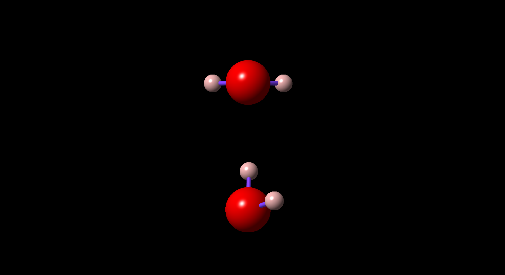

$d=10$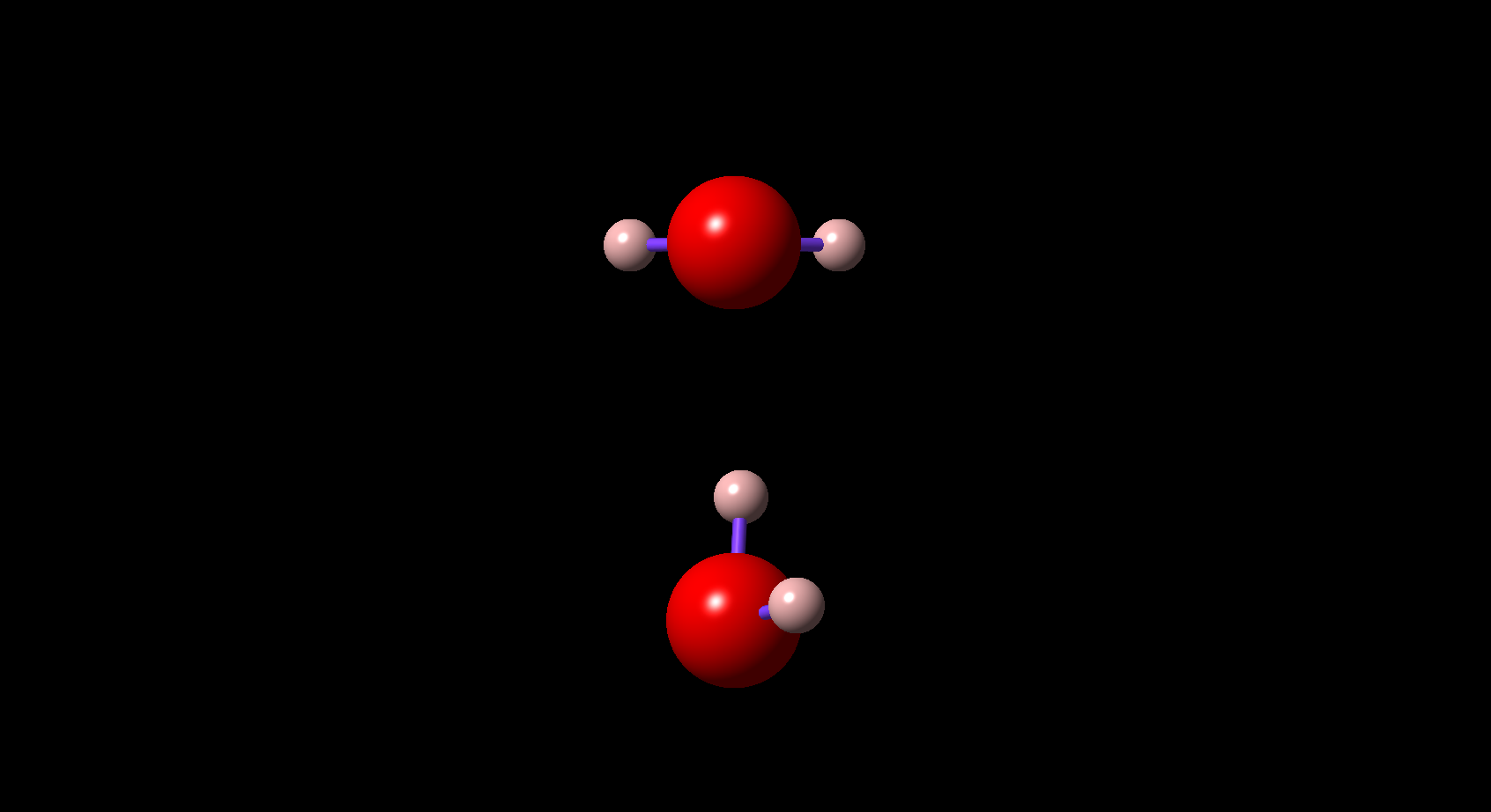

$d=20$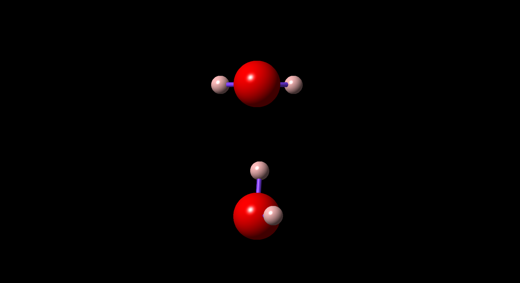

$d=30$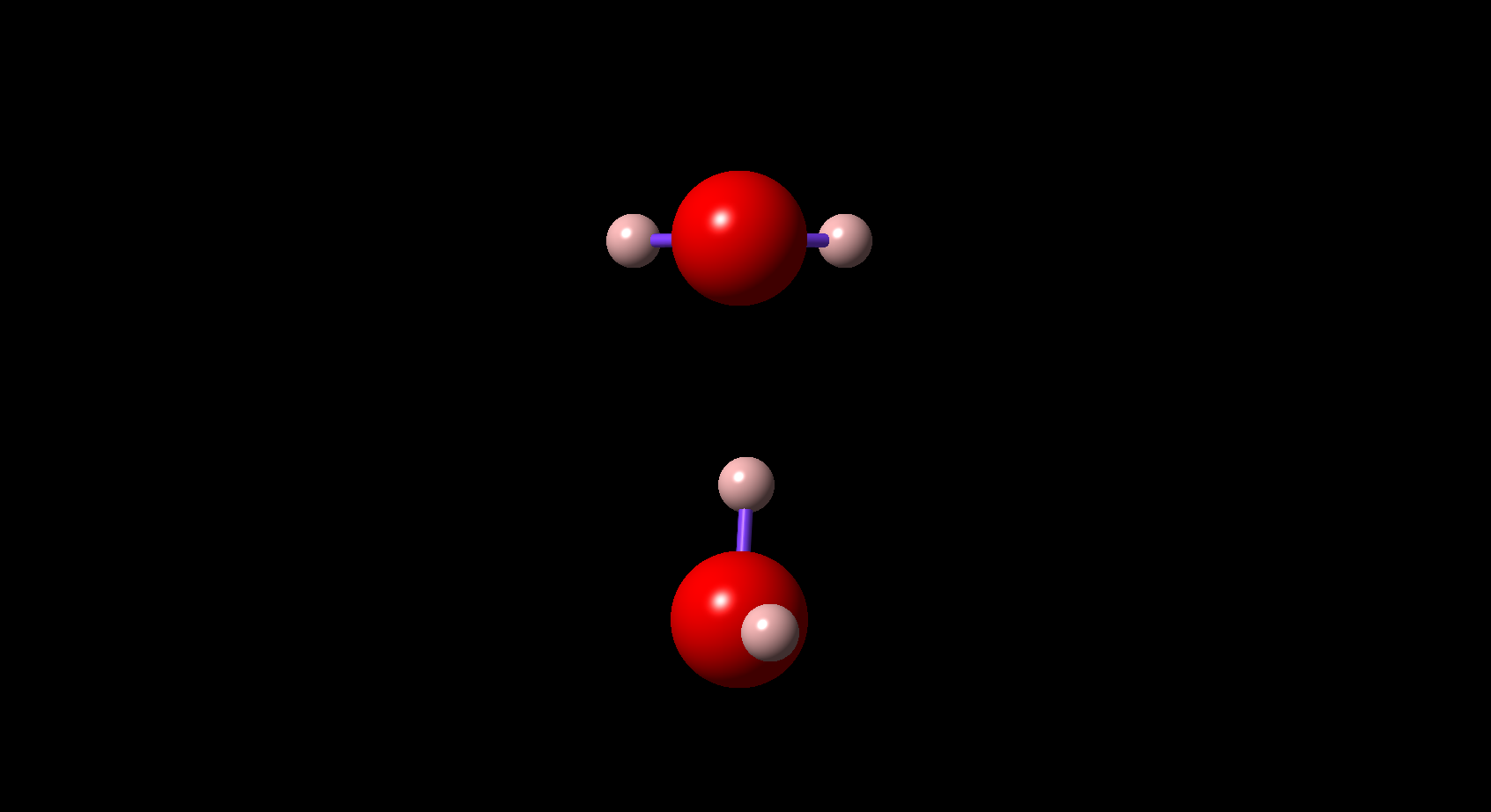

$d=40$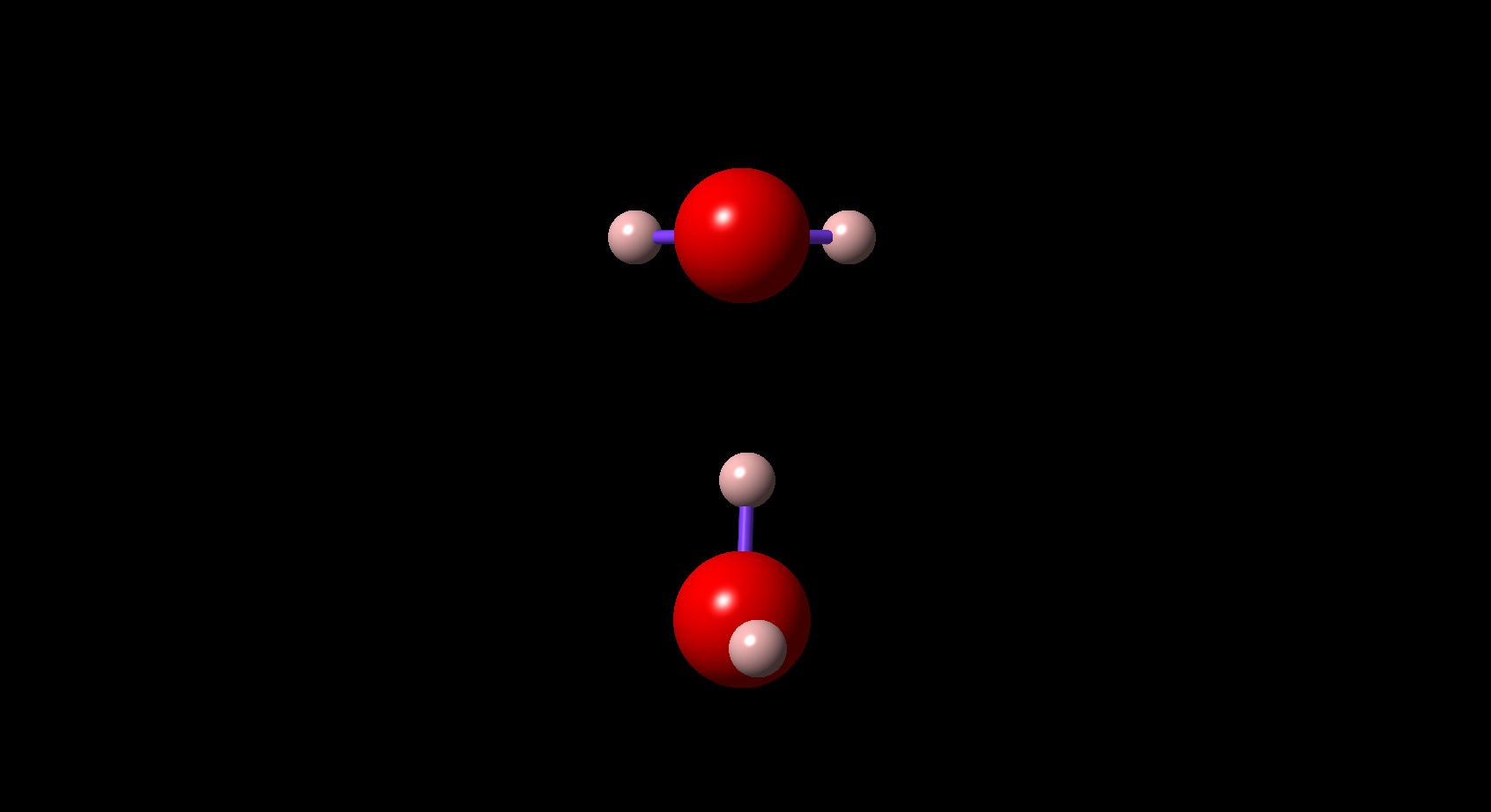

$d=50$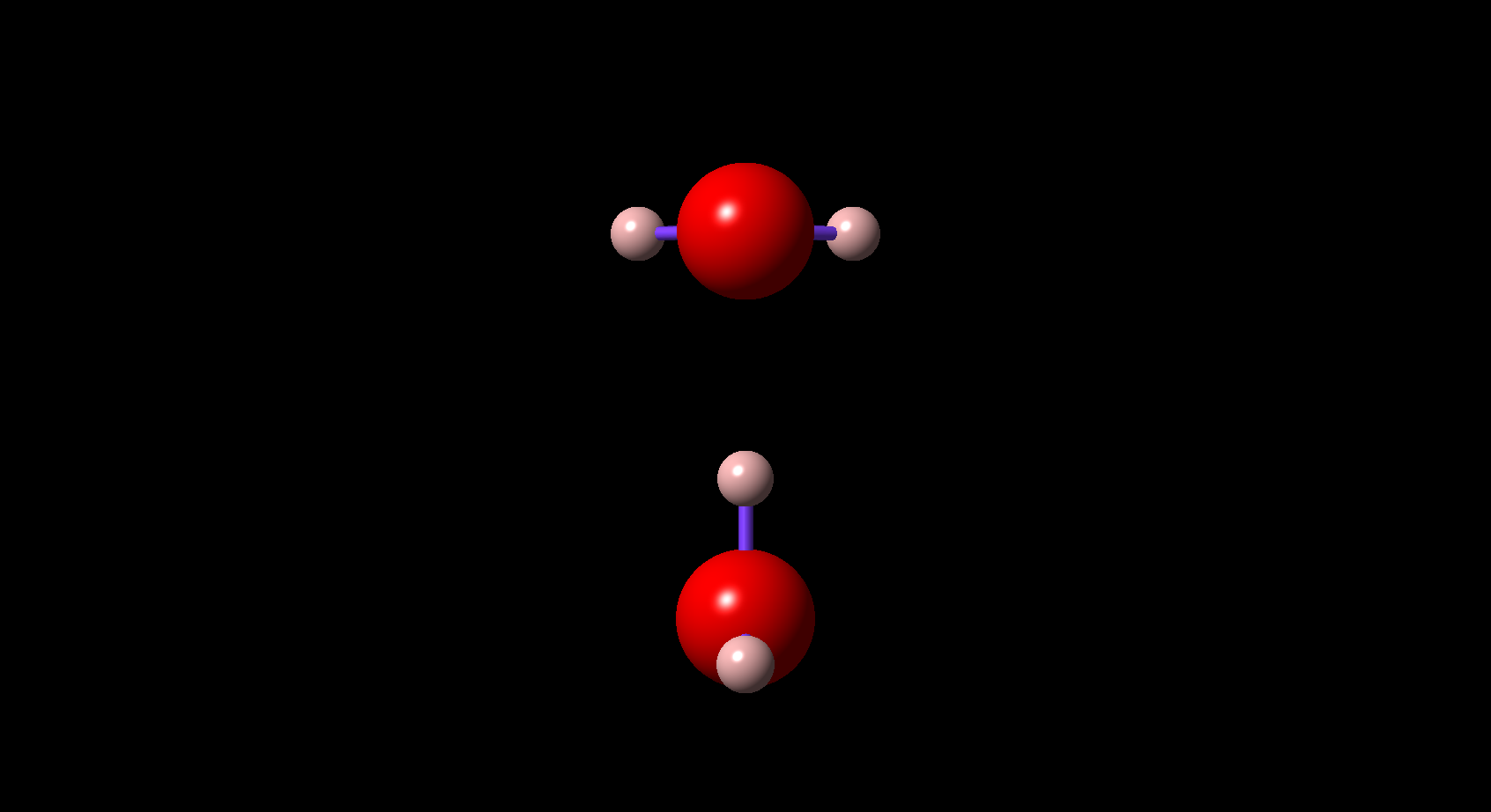

$d=60$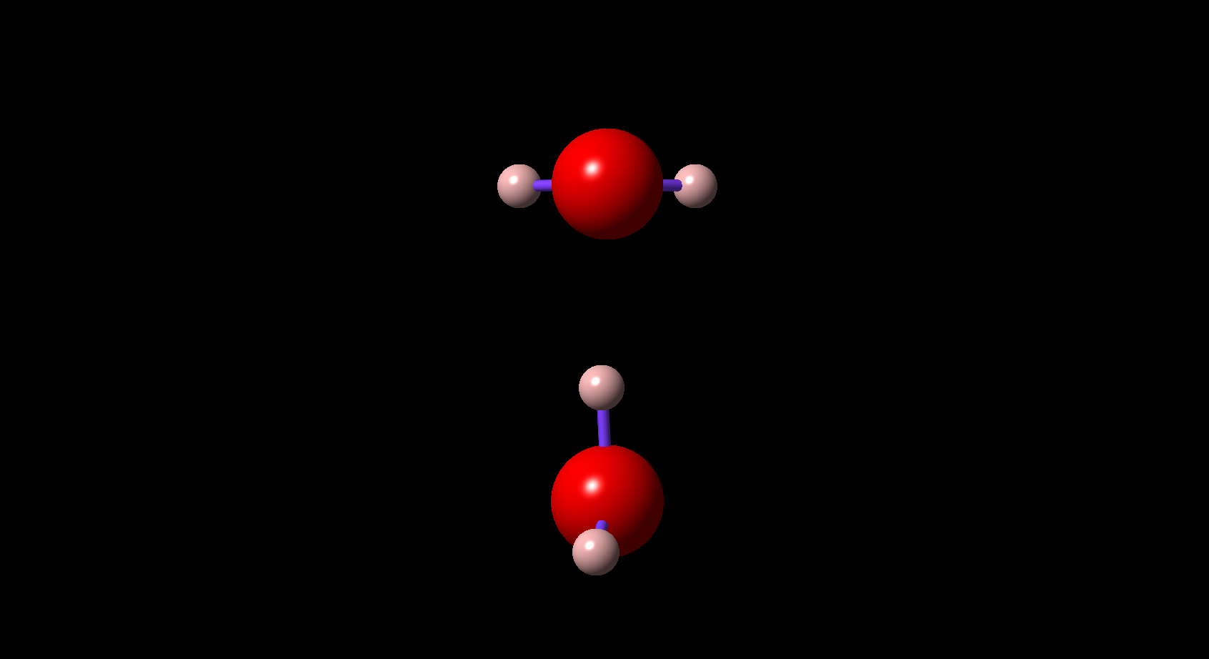

$d=70$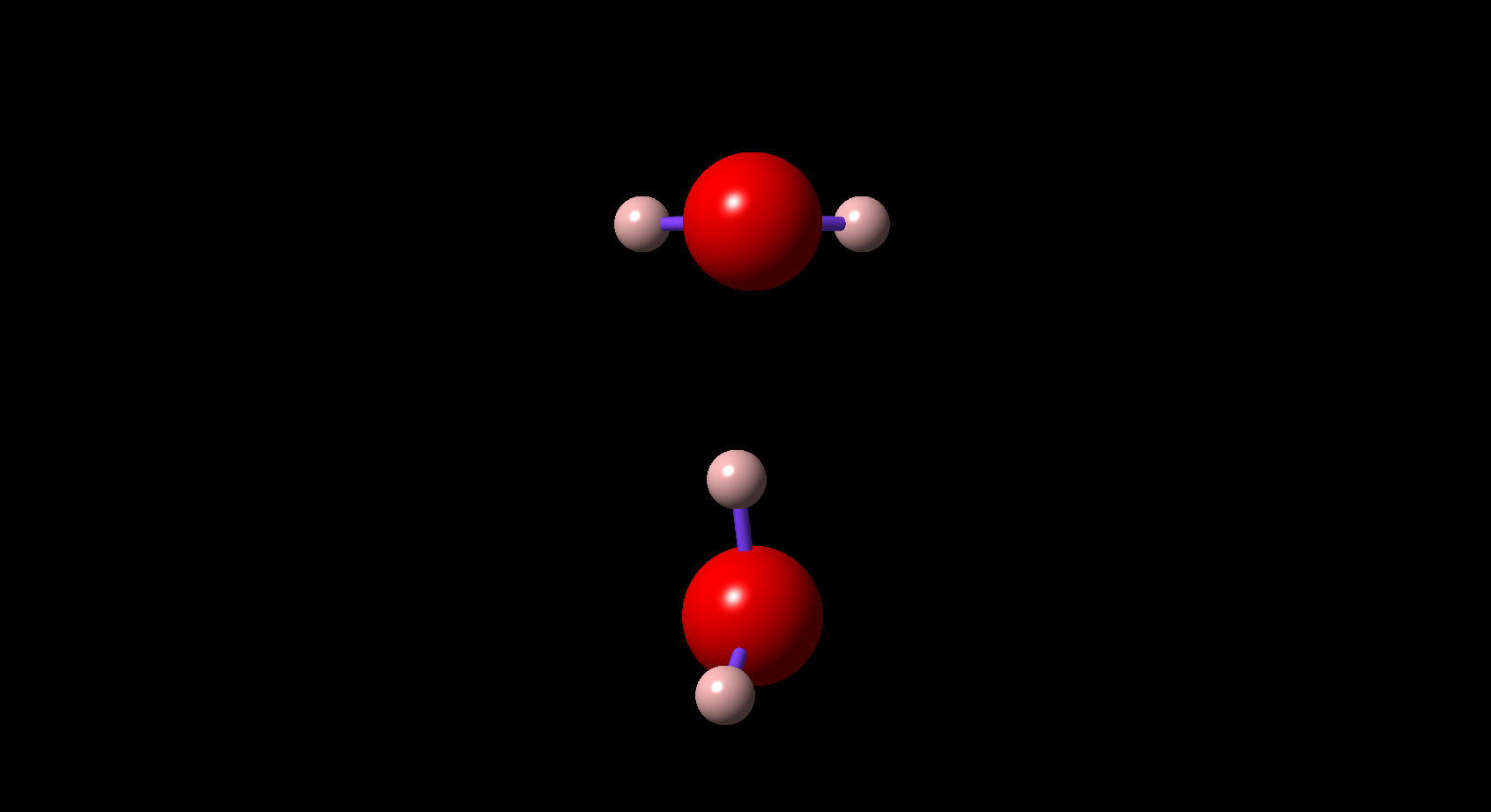

$d=80$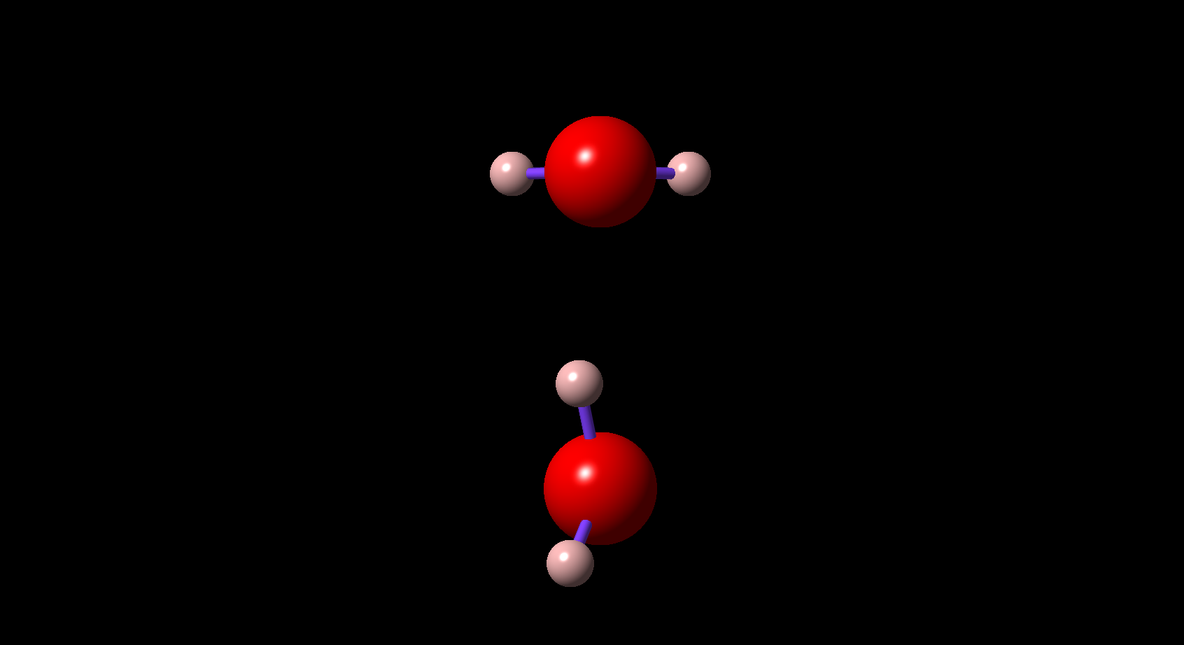

I have the coresponding profile plots of the energy but am having trouble uploading them.